Thermal Systems Part 2

Instead of simulating a cup of coffee heating up, we got to use an actual thermal system today. It consisted of a heater (a 50 ohm resistor) with an 18 V supply, a thermal reservoir, and a temperature sensor.

Deliverable 1
First, we connected our system to the computer and ran a code called test_thermal which turned on the heater for 300 seconds to 100% power and then plotted the temperature as the system warmed up. Here's a picture of that code and the resulting graph.

The next step was to use this graph to find the thermal resistance, Rth, and the heat capacity, C.  We used Rth = delta T / P and the initial (y(1)=310.5602) and final (y(300)=344.6363) temperatures to find Rth = (344.6363 K -310.5602 K)/(6.5 W) = 5.24 K/W.  Then, we used C = P / (dT/dt) to find C. We used data from t=1s to t=11s because that was where the graph could be approximated by a line. We found dT/dt= (T(11)-T(1))/(11-1) = (313.8624 K-310.5602 K)/(11 s-1 s) =  0.3302 K/s. Then we found C = P / (dT/dt) = 6.5 W/0.3302 K/s = 19.68 J/K. The time constant is defined as the time required for the system to reach 63.2% of its final asymptotic value which was about .632*(344.6363 K-310.5602 K)= 21.54 K. By looking at the vector y, we found that the time to reach 310.5602K +21.54K = 332.1 K was about 93 seconds.  Our prediction was tau = Rth*C = 5.24K/W*19.68J/K=103.12 seconds. So, the actual time for the system to respond was less than the expected time.

Deliverable 2
Next, we edited the given code heatsim.m to reflect the newly calculated values, Rth = 5.24 K/W and C = 19.68 J/K, as well as the max power 6.5 W.  We ran this simulation and compared it to to our experimental data.

Here is our modified heatsim.m script.

We wrote this code so that we could plot the simulated and experimental data on one graph. The experimental data is plotted in blue and the simulated data in red. 

The y axis is temperature (K) and the x axis is time (s). In this graph, the experiment looks like it follows the simulation extremely well. 

               

However, when we zoom in by changing the y axis range from 200-500 K to 300-350 K, we can see that it's not as good a match as we thought. The experimental curve is much bumpier than the extremely smooth simulation curve. The experimental curve is pretty smooth until about 75 seconds, but then it starts to fluctuate and deviate farther from the predicted curve. This is because real-world systems don't operate just as ideal, hypothetical systems do. Us touching the reservoir may have caused some fluctuations, and perhaps the power from the heater and other variables aren't as constant as we thought they'd be.

Deliverable 3

Next, we implemented bang-bang control, so that if the system was below the ideal temperature, the heater would run at max power, and if it was equal to or above the ideal temperature, the heater would not run at all. 

Here's the code for our bang-bang simulation. 

And here's the graph.  It doesn't really look like bang-bang to us. It looks too smooth. We decided to zoom in to see if the "bang bangs" would be more visible. 

In the zoomed in version, you can see that the graph levels off at 340 K around 225 s. 

I edited the code so that the simulation would run for 600 seconds, hoping to see characteristic bang-bang behavior. Unfortunately, it stays at 340 K after 225 s. Once the temperature is equal to or less than 340 K, the power should be set to 0, which would cause the temperature to drop, which would cause the power to be turned back on and the temperature to rise. I'm not sure why the simulation levels out at 340 K.

We moved on to our bang-bang experiment, which turned out as expected. Unlike the previous graph, in the experimental graph you can see the variations in temperature as the power is turned on and off.  

Deliverable 4
Next we implemented proportional control so that the power provided by the heater was proportional to the difference between the actual and desired temperature. The farther from ideal the temp was, the more power would be provided by the heater, and the closer to ideal temp, less power would be provided so that it wouldn't overshoot the ideal temperature. Since we can't have a negative power or a power greater than the heater's capabilities, we set the minimum power to 0 and the maximum to 6.5 W.

We worked on this project over several days, using different sensors (we had to switch them out so that we wouldn't have to wait for one to cool down). The sensor we were using while working on proportional control read 300 K as the ambient temp instead of 310 K, so we changed our code to reflect this. However, our Rth and C values were calculated using an ambient temperature of 300 K. This may be one reason for our issues (which are discussed below our graphs).

K = 0.05

K = 0.2

K=0.5 

As you can see, the greater the K value, the h the higher the final asymptotic temperature. However, even when when we made K ridiculously large, the temperature never reached the ideal of 340 K. The only way we could reach a temp of 340 K is if we added a constant to our power equation. For the graph below, we used the equation P = 5 + k*error with k = 0.5. We thought these constants were optimal, so we also used them for our experiment.

K = 0.5, P = 5 + K*error

Note that this simulation starts from an ambient temperature of 310 K because we'd been using our sensor since we ran the last simulations and it hadn't cooled down completely. 

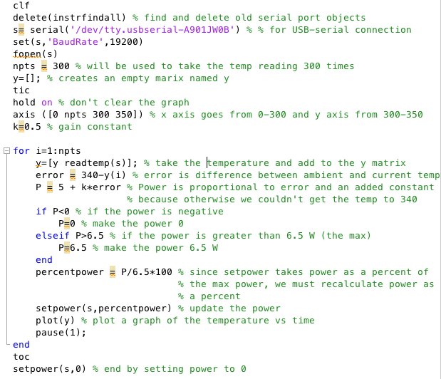
Here is our code for our experimental proportional control. This code differs from the simulation code because the heater power has to be set as a percentage of the max power. Therefore, after we calculated the power, we divided by 6.5 W and multiplied by 100 to find the percentage.

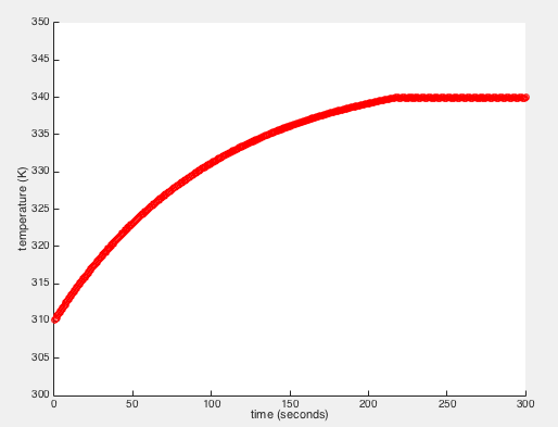
K = 0.5, P = 5 + K*error

Compared to our simulation, this graph seems to level off a bit sooner, around 100 s, and it's also a lot bumpier, due to factors not accounted for in the simulation. However, the simulation is overall a pretty good fit.