MatLab

This week we learned MatLab, which I was very excited about because my graphing calculator just broke.

Exercise 2.1 Our first exercise was to write a program that could compute the nth Fibonacci number, and then find the 10th Fibonacci number. This was as simple as inputting the given equation (being careful with placement of parentheses) and setting n=10 before running the program. Here is the code.

When we set n=10, the answer was 55, just like it should be!

Exercise 2.3 Imagine that you are the owner of a car rental company with two locations, Albany and Boston. Some of your customers do “one-way rentals,” picking up a car in Albany and returning it in Boston, or the other way around. Over time, you have observed that each week 5% of the cars in Albany are dropped off in Boston, and 3% of the cars in Boston get dropped off in Albany. At the beginning of the year, there are 150 cars at each location. Write a script called car update that updates the number of cars in each location from one week to the next. The precondition is that the variables a and b contain the number of cars in each location at the beginning of the week. The postcondition is that a and b have been modified to reflect the number of cars that moved.

Here is my attempt at solving this problem. After one week, A had 147 cars and B had 153 cars. However, I found out that this solution is wrong because it violates the "conservation of cars." A updates in the first line, so then the second line uses the new A to update B instead of the old A. After a while, this throws off the total number of cars so that it's less than 150, which doesn't make sense. This is a good lesson that in MatLab, you need to try several different calculations with your program (in this case, checking the number of cars after several weeks instead of just after the first) to make sure everything makes sense. 

This code works because it uses the old a and b to update the new a and b. Round is used because otherwise you get fractions of cars, which just doesn't make sense. If you check a few weeks, you can see that the number of cars always equals 300.

Exercise 3.1 Create a script named car loop that uses a for loop to run car update 52 times. Remember that before you run car update, you have to assign values to a and b. For this exercise, start with the values a = 150 and b = 150.

In order to see the number of cars in each location at the end of the year, I used a for loop that updates a and b 52 times, since there are 52 weeks in a year. At the end of the year, there were 118 in Boston and 182 in Albany. Since this code ran 52 times, it displayed a lot of numbers on the screen, which was overwhelming. A graph would be useful for interpreting this data.

Exercise 3.2 Modify car loop so that each time through the loop it plots the value of a versus the value of i.

Here is the code that plots a vs. i and its corresponding plot. You can see that at week 21, the number of cars in Albany becomes stable at 118. You can also see that when you don't specify a color for your circles, MatLab automatically alternates colors.

b. Once you get that working, modify it so it plots the values of a with red circles and the values of b with blue diamonds.

Here is the code that plots the values of a and b vs. i and its corresponding plot. You can see that at week 21, equilibrium is reached. There are 118 cars in Albany and 182 in Boston. One thing you have to be careful about in MatLab is clearing your workspace. At one point my a vs. i graph showed equilibrium occurring at week 17, whereas my a and b vs. i graph showed equilibrium at week 21. This is because I hadn't cleared my workspace before running the first program and it was starting with initial a and b values other than 150.

I also tried making a plot with initial a and b values of 10000. It looks parabolic!

Exercise 3.5 We have already seen the Fibonacci sequence, F, which is defined recurrently as Fi = Fi−1 + Fi−2. In order to get started, you have to specify the first two elements, but once you have those, you can compute the rest. The most common Fibonacci sequence starts with F1 = 1 and F2 = 1. Write a script called fibonacci2 that uses a for loop to compute the first 10 elements of this Fibonacci sequence. As a postcondition, your script should assign the 10th element to ans.

It's been a while since I thought about recursive sequences, let alone coding with them, so this one took a few tries. I checked that this code worked by googling the Fibonacci sequence and comparing it against my answers. The 10th Fibonacci element calculated was 55.

b. Now generalize your script so that it computes the nth element for any value of n, with the precondition that you have to set n before you run the script.

Exercise 4.6 The ratio of consecutive Fibonacci numbers, Fn+1/Fn, converges to a constant value as n increases. Write a script that computes a vector with the first n elements of a Fibonacci sequence (assuming that the variable n is defined), and then computes a new vector that contains the ratios of consecutive Fibonacci numbers. Plot this vector to see if it seems to converge. What value does it converge on?

For this plot I used n=100. The plot starts at i=2 (point (2,1) which is the ratio of the second element to the first element) since i=1 would correlate with the ratio of the 1st element to 0th element, and there's no 0th element. The plot definitely converges, and if you check the printout of the ratio vector, you can see that it converges at 1.618. A google search told me that the ratio of Fibonacci numbers indeed converges at 1.618, which is called the golden ratio.  For reference, here is the printout of the vector where the ratios were stored.

R =

  Columns 1 through 12

    1.0000    2.0000    1.5000    1.6667    1.6000    1.6250    1.6154    1.6190    1.6176    1.6182    1.6180    1.6181

  Columns 13 through 24

    1.6180    1.6180    1.6180    1.6180    1.6180    1.6180    1.6180    1.6180    1.6180    1.6180    1.6180    1.6180

  Columns 25 through 36

    1.6180    1.6180    1.6180    1.6180    1.6180    1.6180    1.6180    1.6180    1.6180    1.6180    1.6180    1.6180

  Columns 37 through 48

    1.6180    1.6180    1.6180    1.6180    1.6180    1.6180    1.6180    1.6180    1.6180    1.6180    1.6180    1.6180

  Columns 49 through 60

    1.6180    1.6180    1.6180    1.6180    1.6180    1.6180    1.6180    1.6180    1.6180    1.6180    1.6180    1.6180

  Columns 61 through 72

    1.6180    1.6180    1.6180    1.6180    1.6180    1.6180    1.6180    1.6180    1.6180    1.6180    1.6180    1.6180

  Columns 73 through 84

    1.6180    1.6180    1.6180    1.6180    1.6180    1.6180    1.6180    1.6180    1.6180    1.6180    1.6180    1.6180

  Columns 85 through 96

    1.6180    1.6180    1.6180    1.6180    1.6180    1.6180    1.6180    1.6180    1.6180    1.6180    1.6180    1.6180

  Columns 97 through 99

    1.6180    1.6180    1.6180

For our final exercise, we were given a script that calculates and plots the path of a projectile launched at a 30 degree angle with an initial speed of 50 m/s. We were then asked to expand on the code in order to find the angle at which the range was maximized. One option would be to manually run the simulation for all angles from 1 to 90, find the maximum range, and identify the angle that produced it. However, we interpreted the instructions to mean that we should write one script that will return as the answer the angle that produces the maximum range. This turned out to be a time consuming and difficult task, but we got an answer pretty close to 45, which is what we know the answer should be.

This script came up with an answer of 48. Here is a printout of the vector Ranges, which collected the range for each angle.

Ranges =

  Columns 1 through 13

   34.9947   39.9756   44.9383   54.8660   59.7717   69.6165   74.4410   84.1728   93.8304   98.4808  107.9790  117.3777  121.7963

  Columns 14 through 26

  130.9899  140.0592  144.1893  153.0088  161.6796  165.4658  173.8431  182.0482  185.4368  193.3060  196.4123  203.9193  211.2166

  Columns 27 through 39

  213.8416  220.7369  223.0280  229.4967  231.4352  237.4535  239.0211  244.5661  245.7456  250.7953  251.5702  256.1035  256.4582

  Columns 40 through 52

  256.6249  260.3748  260.1007  259.6306  262.5590  261.6295  260.4969  259.1594  260.9609  259.1433  257.1150  254.8748  252.4212

  Columns 53 through 65

  249.7532  246.8698  243.7700  240.4529  236.9180  233.1645  229.1919  225.0000  220.5884  215.9569  211.1056  203.8426  198.6306

  Columns 66 through 78

  193.1999  187.5509  179.8112  173.8085  167.5899  159.5284  152.9634  144.7240  137.8187  129.4095  122.1706  113.6003  106.0350

  Columns 79 through 90

   97.3126   88.5606   79.7816   71.6741   62.7627   53.8322   44.8852   35.9246   27.2147   18.1477    9.0753    0.0000

Based off this data, you can tell that there are several problems. An angle of 45 degrees should produce the maximum range, according to my physics knowledge. This script shows an angle of 45 degrees producing a range of 261.6295. However, 44 degrees produces the largest range, 262.5590. The program picks 48 degrees, with a range of 260.9609, as the range-maximizing angle. I think this may have something to do with the fact that after angle 48, the ranges gradually decrease, but before angle 48, the ranges do not gradually increase. The behavior is like this: ...<R(41)>R(42)>R(43)<R(44)>R(45)>R(46)>R(47)<R(48)>... Obviously, something weird happens with the math in the 40s, and because of the way my program is written, 48 is picked as the range-maximizing angle since the ranges steadily decrease after that.  I'm left with two questions: why is 44 the true range-maximizing angle, and how can I get my script to pick 44 as the range-maximizing angle?

SciBorg Part 2 (Drive Straight, Follow the Line, Follow Another SciBorg)

Drive Straight

Our next task was to implement bang-bang control to make the SciBorg drive straighter. We wrote a program that only gave the SciBorg three options: drive with both motors at the same fixed speed, make a gentle left turn, or make a gentle right turn. We decided to use the motor encoder for this task to determine which direction the SciBorg was straying. If the position of motor 2 (the left motor) is greater than that of motor 1, that means motor 2 is travelling faster, so the SciBorg is turning right. This must be corrected with a gentle left turn. We defined a gentle left turn as motor 1 speed 5 faster than motor 2 speed. If the position of motor 1 (the right motor) is greater than that of motor 2, that means motor 1 is travelling faster, so the SciBorg is turning left. This must be corrected with a gentle right turn. We defined a gentle left turn as motor 2 speed 5 faster than motor 1 speed. If both motors are at the same position, the SciBorg is driving straight, so nothing should be done (that is, both motors should continue at the same speed).  Here is a picture of our code and videos of the SciBorg travelling on different surfaces. 

On the Lab Floor

The SciBorg goes straighter, but it's obviously not perfect. Towards the end, you can see that it's veering to the left. 

On the Carpet 

There's more friction on the carpet, so you can see the SciBorg shaking a bit. It also appears to veer right in the beginning and left towards the end. 

Going Up the Ramp

As you can see, the SciBorg veers to the right and falls off the ramp pretty quickly.

Going Down the Ramp

The SciBorg veers to the left and falls off the same side of the ramp as when it was going up. This made us think that the ramp was crooked or provided different friction forces to the two wheels. The SciBorg appeared to make it farther down the ramp before falling off than it did up the ramp.

Conclusion

It's very difficult to get the SciBorg to drive straight. Its path depends greatly on the surface it's driving on, but it seemed to do best on the lab floor. The various surfaces certainly all provide different frictional forces, which probably affects its path. I wonder what the coefficients of friction are for each of the surfaces and what the optimal coefficient is. I also wonder what the coefficient of friction between rubber car tires and asphalt is. It also may not be entirely the surface's fault that we could never get our car to drive straight. Perhaps we had a fault in our logic. I'm not sure if the assumption that equal motor positions means the car is going straight is true. The differences in speed between the two motors can be inconsistent, and the way we defined our gentle turns was pretty arbitrary. I'm thinking that perhaps if the SciBorg veers to the left (with a natural speed difference between the motors that is greater than or less than 5)  and we try to correct it with a gentle right turn (with a programmed speed difference of 5), maybe when the motor positions become equal again, it won't necessarily be pointing straight. I don't think using the motor encoder with this strategy was the best way to make the SciBorg drive straight. We had a couple other ideas: First, put a straight line of white tape down and, using the light sensor, program the SciBorg to follow the line. Second, put a narrow delrin board 2 feet behind wherever you want the SciBorg to stop (as documented in my last blog post). Put another delrin to the left and 1 foot behind the first delrin board. Put a third delrin board to the right and 2 ft behind the first board. This way, the three boards are staggered, and the ultrasonic sensor would have different readings depending on which one it was pointing at. Then, you could program the SciBorg to make a gentle right turn if the ultrasonic sensor reading was consistent with facing the left delrin board, or make a gentle left turn if it was facing the right board. However, both of these methods are pretty complicated and involve augmenting the lab floor course, which I'm not sure if we were allowed to do. I feel like there must be a better way that we haven't thought of yet. 

Bang-Bang Line Following

Our next challenge was to use our brightness sensor to make our Sciborg follow a zigzagging line. We tried for a very long time with no success to get this to work. Finally, we came to the realization that using while loops to make the SciBorg follow the edge of the white line would be our best bet. We found that the edge of the white line had a brightness reading in the 80s (depending on how much white vs. brown was under the sensor), so we decided to use a value of 80. We coded the SciBorg so that while it saw a brightness of less than 80 (meaning it's over wood), it should make a hard left. Once it sees a brightness of greater than 80 (meaning it's over the white tape), it should make a hard right, and then repeat the loop. (Note: In the code below, we accidentally named the right turn left and the left turn right!) The trickiest part was fine-tuning the speeds of each motor in the turn definitions. The turns had to be hard enough that the SciBorg could handle the sharp turns on the course. Here is a picture of our code and a video of our SciBorg following the line. 

Follow Things

Our final challenge was to make our SciBorgs follow each other in a line. We wrote a program using the ultrasonic sensor that told the SciBorg to drive if the object in front of it was more than 2 feet away, and stop otherwise. We used an ultrasonic reading value of 37 to correspond to an object 2 feet away (details in my last blog post). Here is a picture of our code and videos of our SciBorg following me and another SciBorg. 

Following Me

Following Another SciBorg

This was pretty neat! It was easier to make the SciBorg follow me because I could sense when it was veering and adjust my position so that it would continue following me. Even though the SciBorgs didn't drive completely straight, they still stayed in line for quite some time.

SciBorg Part 2 (Sensors and Stopping After 5 Feet)

Our first challenge was to explore different sensors (an ultrasonic sensor, a light sensor, a motor encoder, and a switch) to understand how they work, and then use each sensor to make our SciBorg travel a predefined distance and then stop. We then analyzed the advantages and disadvantages of each sensor and came to a conclusion about which was most effective.

Motor Encoder

The first sensor we tried out was the motor encoder, which reports the position of the motor at a specific time. We ran a program which made motor 1 repeatedly spin forwards at speed 225 for 1 second, then spin backwards at speed 225 for 1 second. The program printed out the position of the motor at the end of each loop (once per second). One would expect the motor to spin forward x amount, so that the first position recorded is x, and then spin a distance of -x, so that the 2nd position recorded is 0 (x-x=0). However, as you can see in the picture of the printouts below, this was not the case. The motor is inconsistent, so it doesn't always spin the same distance in the same amount of time. That is, the speed you assign to the motor in the code isn't always the speed it actually goes. In addition to inconsistencies on the motor's part, perhaps the voltage from the USB port fluctuates slightly, which results in slightly different speeds. 

You can see how inconsistent one motor is, imagine trying to get two of them to work together! Next, we ran a program that printed out the positions of both motors after each second. We noticed that motor 1 was much slower than motor 2. We thought it would be interesting to plot the relationship. Below, you can see that the difference in motor position vs. time fits a quadratic relationship. We thought that perhaps we could use the equation generated to determine how much to adjust the speeds of the two motors in order to make the SciBorg drive a straight line. That's definitely not bang-bang control, though, so we'll save it for another time.

Next. we programmed our SciBorg to move forward at speed 225 and timed how long it took to travel 5 ft, which was 8 seconds. We then plugged it into the computer and read the positions of the two motors after 8 seconds. We did this several times. The average position of the slowest motor (motor 1) after 8 seconds was 6123. We then wrote a program that told the SciBorg to move forward at speed 225, and stop when the position of motor 1 was equal to or greater than 6123. Here is our code.

Here is a video of our SciBorg running the code. 

Our SciBorg stopped about 3-4 inches short of the 5 foot mark, which I think is pretty good. It stopped shorter than 5 feet because of the value we used for the stopping position, 6123. This value was an average, so depending on the trial, the motors may travel farther or less in 8 seconds. In the case shown in the video, the SciBorg was a little on the faster side, which is why it reached position 6123 sooner and stopped shorter than we hoped.

Touch Switch

The next sensor we experimented with was the tactile switch. I think this sensor was the easiest to use. When the button is unpressed, electricity can flow to the specified pin, so a reading of that pin would be high. When it is pressed, electricity flow is reduced to the specified pin, so a reading of that pin would be low. We used the values read from the pins to determine whether our car should stop or go. We placed a large piece of delrin at the 5 foot mark, supported by a trash can. The SciBorg should travel until it runs into the delrin, pushing the button and causing a pin reading of low, which tells the SciBorg to stop moving.  Below is a picture of our code and a video of our result. 

This method was extremely accurate for making the SciBorg stop after 5 ft. However, it is pretty inconvenient, because you'd probably want to be able to stop a vehicle without having to place a large obstacle in front of it. Also, depending on how fast a hypothetical vehicle is travelling, running into something in order to stop could cause damage.

Light Sensor

Next, we experimented with the light sensor. We ran a program which printed the values detected by the light sensor in order to understand which surfaces had high, moderate, and low values of light reflection. Here is a video (without the LED light turned on) in which you can see the values detected for different surfaces. 

When we turned on the LED, the sensor picked up values in the 90s for pretty much every surface we put under it. We couldn't really figure out what the LED is good for, besides showing you exactly where on the surface the sensor is reading from. Below is a video with the LED light turned on in which you can see the values detected for different surfaces. 

We noticed that the readings are more accurate when the sensor is closer to the surface (but not pushed up against it, as this blocks out light and can make a bright surface appear dark), so we attached the sensor on the car so that it would be very close to the ground.

Since the lab floor is gray, it has a relatively low value of light reflection. White paper had values in the high 90s. We put a white paper on the 5 ft mark on the lab floor. Then, we wrote a program that told the SciBorg to drive if the light reflection value was less than 90, and stop otherwise. Here is our code and a video of our result. 

The light sensor method was very effective. As you can see in the video, the SciBorg stopped almost immediately after it reached the white paper at the 5 ft mark.

Ultrasonic Sensor 

The last sensor we worked with was the ultrasonic sensor. This sensor emits sound waves which hit the nearest surface in front of the SciBorg and reflect back. The sensor measures how long it takes to receive the reflected wave back, which is used to calculate the distance to the obstacle. As the handout states, "because of acoustic phase effects in the near field, objects between 6-inches and 20-

inches may experience acoustic phase cancellation of the returning waveform resulting in inaccuracies of up to 2-inches. These effects become less prevalent as the target distance increases, and has not been observed past 20-inches. '' We decided to escape this issue by writing a program that makes the SciBorg stop when it's 2 ft away from an object. When the delrin was 2 ft from the SciBorg, the sensor read a value of about 37. We used a distance less than this value (if distance < 37) as the stopping point for our program and placed a delrin sheet 2 ft from the 5ft marker on the floor. A picture of our code and a video of our result appear below.

The ultrasonic sensor ended up being about 1.5 inches from the 5 ft mark. Pretty good, but once again, using this sensor was a little more complicated than it was worth. 

Conclusion

The tactile switch and the light sensor had the highest accuracies for stopping at the 5 ft mark. The tactile switch was the easiest to use/program for, and the light sensor was a close second. The motor encoder and the ultrasonic sensor were both inaccurate and difficult to use. 

Real-world Feedback and Control Systems

What are four examples of feedback/control systems you encounter in your everyday environment?

1. Swipe access doors
Sensor- A sensor reads the magnetic strip on a OneCard.
Control mechanism- If the sensor determines that the code written on the magnetic strip has access, a signal is sent to the actuator to unlock the door. Otherwise, no signal is sent.
Actuator- The mechanism that provides the energy to unlock the door. (A motor?)
What works well: The door only opens if it reads a card with access, so other people can't get in. The door doesn't stay unlocked for very long. This way, people without access can't sneak in after you.
What Doesn't Work Well: Sometimes the reader doesn't read the card and you have to swipe more slowly or swipe twice.

2. Handicap doors 
Sensor- The button on the wall near the door is the sensor.
Control mechanism- When the button is pushed, a signal is sent to unlock the door.
Actuator- The mechanism that provides the energy to unlock the door. (A motor?)
What works well: Very effective. I've never seen a door fail to open when the button is pushed.
What Doesn't Work Well: People use it just because they're lazy and therefore waste energy. The door stays open for a long time, so people who don't have access can get inside.

3. Ionization smoke detectors
The battery in the smoke detector sends voltage to plates, making one positive and one negative. A radioactive isotope in the detector decays at a constant rate and emits alpha particles.  They ionize with the air flowing through the chamber in order to create a constant current between the two plates. When the air flowing through the chamber has particles or water vapor in it, it can interrupt the current.
Sensor-The sensor measures the current flowing in the chamber.
Control mechanism- If the sensor measures a current lower than expected, it signals the actuator.
Actuator- The battery sends an electric pulse to the electromagnet in the speaker, which then vibrates and creates sound.
What works well: It's very effective, beeps to warn residents that the battery is low
What doesn't work well: It can be triggered by steam from boiling water or a shower.

4. Stove/Oven Timer
In the dorm kitchens we have timers connected to the oven and stove that we must turn in order to use the stove or oven.
Sensor- Something senses whether the timer is at 0. I think it might be a tactile switch. After you twist the timer on, it slowly ticks back to 0 until a part taps the switch.
Control Mechanism- When the switch is triggered, a signal is sent to turn off the flow of electricity to the oven and stove.
Actuator- Wherever the electricity for the oven and stove comes from. When it's turned off, turning the oven to bake or the stove to high doesn't do anything. You must turn the timer to allow the electricity to flow again.
What works well: The timer prevents people from accidentally leaving the stove or oven on for long amounts of time and therefore increases the fire safety of the building.
What doesn't work well: The timer is really short so if you're trying to bake a cake or something, the oven will turn off in the middle and you'll have to restart it. This is especially bad if you don't realize it turned off and then find a pan of batter when you expect to find a cake. You should be able to set the timer for as long as you need.

Sciborgs Day 1

Our first task was to write a sketch that makes an LED flash the Morse code for SOS using functions to reduce repetition.  Here is our commented code.

Next, we had to set up the Sciborg. Our first Sciborg task was to download the code "single motor" from the class website and run it to see what it does. Our commented code and a video of the Sciborg after uploaded the program appears below. One problem we had was that gibberish was appearing in the printing window. We had to make sure to change the data rate in the printing window.

Challenge 1: Create a new sketch, based on the previous sketch, to run both motors simultaneously at the same speed. A picture of our code and a video of the result appears below. 

Challenge 2: What is the minimum speed that allows your Sciborg to move? For this task, we basically had to guess and check by entering different speeds and then running our program to zoom in on the minimum speed. We defined the minimum speed as a speed at which the Sciborg will move without eventually stopping (unless the program says to). We found the min speed to be about 85. A picture of our code and a video of the Sciborg appears below.

Challenge 3: Make a sketch that gets the Sciborg to make a hard turn. We accidentally overlooked the comment that said to accomplish this by making one motor full power forward, the other full power reverse. We instead accomplished this task by making both motors go the same direction, but one at a faster speed than the other. A picture of our code and a video of the Sciborg appears below.

Challenge 4: Make a sketch for making a gentler turn. We accomplished this by making a less dramatic speed difference between the two motors. A picture of our code and a video of the Sciborg appears below.

Challenge 5: Time how long it takes for the Sciborg to travel 10 feet. Write a sketch that makes the Sciborg travel for this much time and then stop. This was the most challenging task. Since there was too much friction with the floor for our Sciborg, we used 9 ft of the table for this task, Our Sciborg had something wrong that caused it to veer left when it was supposed to drive straight, We tried to counteract this by increasing the speed of the left motor, but the behavior was very erratic, and we could never get it to drive straight, Thus, it took a different amount of time each trial to reach the 9 ft mark. Once we decided on the best time value we could get and programmed it into the Sciborg, it would always stop right before the line or right after, depending on how much it deviated from a straight path. A picture of our code and a video of the Sciborg appears below.

Arduino Practice Day 2

Challenge: Use the photocell to change something about the LED behavior based on room brightness.

Our Program

(I'm sorry, but I can't get these photos to line up properly.)

Our Hardware

Our Results

Challenge: Use the tiny tactile switch to turn the LED on and off.

Our Program

Our Hardware

Our Results

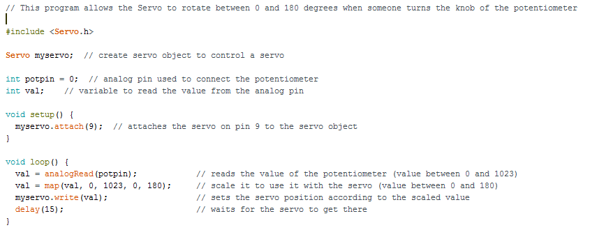
Challenge: Use Knob to control your servo.

Our Program

Our Hardware

Our Results

Challenge: Use Sweep to control your servo

Our Program

This program allows the servo to rotate independently from 0 to 180 degrees.

Our Hardware

See picture for Knob hardware

Our Results

Challenge: Change Knob so the servo only rotates between 60 and 120 degrees.

Our Program

Our Hardware

See picture for Knob Hardware

Our Results

Reflection:

My favorite challenge was the photo cell. First, we established values for different brightness levels by changing the environment of the photocell. For example,  we went in the bathroom and turned the light off to determine a value for dark of less than 100. For very bright, Amy shined her flashlight on the photocell in order to obtain a value of greater than 800. After deciding on all of our values, we programmed the code so that different LEDs would light up depending on the brightness level. I thought that was very neat. 

One frustrating aspect arose when I was trying to run Button in order to take a video. I couldn't get it to work, and I thought that I had put some of the wires in the wrong places. I kept taking the circuit apart and putting it back together, to no avail, I finally realized that the reason it wasn't working was that I was running the Button program from the examples, rather than the code from the handout. 

While I didn't think Servo and Knob were as remarkable as the photocell challenge, I can see how they would be very useful. I was also surprised at how hard it was to stall the servo motor -- neither of us could do it! It must be a very high torque motor. 

Arduino Practice

Challenge 1: Blink with Delay of 10

Our program

Our Hardware/The Result

The LED flashes every 10 seconds but appears as a continuous light because the human eye cannot perceive flashes that happen that quickly. 

Challenge 2: Pattern with 3 LEDs Using Delay() Function

Our Program 

Our Hardware 

The Result (Turning from 0 V to 5 V)

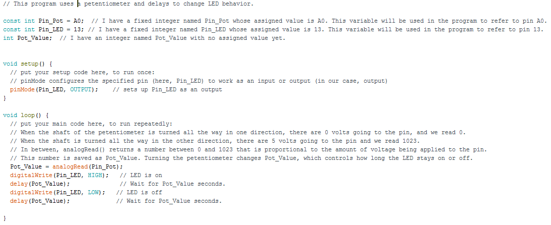
Challenge 3: Use Potentiometer to Change LED Behavior

Our Program 

(You might need to zoom in for this one, this was the largest size possible)

Our Hardware

Our Results (Turning from 0 V to 5 V)

Challenge 4: Pattern with 3 LEDs That Does Not Use Delay() Function

Our Program 

Our Hardware

Our Results

Conclusion:

Working with the Arduinos was a lot of fun. I've taken Python before, and I thought the Arduino programming language was pretty easy to catch onto. I've always been confused by how breadboards work, though, so I was happy to get some more practice with them. I think figuring out where the connections should go and why is the most challenging part. I was also confused at first by what the the potentiometer does, but I found out online that turning it controls the voltage going to the pin. I enjoyed changing the programs and observing the effect in order to understand what each line of code does. I also liked creating the lighting patterns for the LEDs.